Note
Go to the end to download the full example code.
Reproducing Bullock et al. (2022) Assessment Framework
In this example, we reproduce the timeliness assessment framework introduced by
Bullock et al. (2022) using the nrt-validate package. We use the test
dataset provided in the original paper’s supplementary materials.
Data Transformation
The original study requires input data in the form of relative timing (e.g., the
number of days between an actual change and a system alert). In contrast,
nrt-validate is designed to work with absolute dates (e.g., timestamps).
To make the original data compatible, we establish a mock starting date
(base_date) and add the relative lags to it to simulate real calendar dates.
Methodological Differences
There is a key difference in how User’s Accuracy (Precision) is calculated
between the original paper’s code and nrt-validate. This difference comes
down to what is included in the denominator:
Original Approach (Dynamic Denominator): The total number of alerts evaluated grows as the time lag increases. A delayed alert is simply ignored when calculating User’s Accuracy at shorter lags, and is only added to the denominator once the evaluation lag reaches the alert’s delay.
nrt-validate Approach (Fixed Denominator): The denominator for User’s Accuracy is fixed to the total number of alerts generated by the system over the entire period, regardless of the evaluated lag.
The implication of that fixed denominator approach of nrt-validate is that
alert delay is more strictly penalized at shorter lags. We can therefore expect
slightly lower User’s accuracy and F1 scores at low lags when using that approach.
import numpy as np
import pandas as pd
import matplotlib.pyplot as plt

from nrt.validate.metrics import TemporalEvaluator
from nrt.validate.estimators import SimpleRandomEstimator
1. Loading the Original Simulated Data
We start with the arrays exactly as provided in the Bullock et al. notebook.
# Tolerance window (-30 to 365 days) defines agreement bounds.
tolerance_window = (-30, 365)
lags = np.arange(0, tolerance_window[-1], 10)

map_changes = np.array([1, 1, 1, 1, 1, 1, 1, 1, 1, 1, 1, 1, 1, 1, 1, 1, 1, 1, 1, 1, 1, 1, 1, 1, 1, 1, 1, 1, 1, 1, 1, 1, 1, 1, 1, 1, 1, 1, 1, 1, 1, 1, 1, 1, 1, 1, 1, 1, 1, 1, 1, 1, 1, 1, 1, 1, 1, 1, 1, 1, 1, 1, 1, 1, 1, 1, 1, 1, 1, 1, 1, 1, 1, 1, 1, 1, 1, 1, 1, 1, 1, 1, 1, 1, 1, 1, 1, 1, 1, 1, 1, 1, 1, 1, 1, 1, 1, 1, 1, 1, 1, 1, 1, 1, 1, 1, 1, 1, 1, 1, 1, 1, 1, 1, 1, 1, 1, 1, 1, 1, 1, 1, 1, 1, 1, 1, 1, 1, 1, 1, 1, 1, 1, 1, 1, 1, 1, 1, 1, 1, 1, 1, 1, 1, 1, 1, 1, 1, 1, 1, 1, 1, 1, 1, 1, 1, 1, 1, 1, 1, 1, 1, 1, 1, 1, 1, 1, 1, 1, 1, 1, 1, 1, 1, 1, 1, 1, 1, 1, 1, 1, 1, 1, 1, 1, 1, 1, 1, 1, 1, 1, 1, 1, 1, 1, 1, 1, 1, 1, 1, 1, 1, 1, 1, 1, 1, 1, 1, 1, 1, 1, 1, 1, 1, 1, 1, 1, 1, 1, 1, 1, 1, 1, 1, 1, 1, 1, 1, 1, 1, 1, 1, 1, 1, 1, 1, 1, 1, 1, 1, 1, 1, 1, 1, 1, 1, 1, 1, 1, 1, 1, 1, 1, 1, 1, 1, 1, 1, 1, 1, 1, 1, 1, 1, 1, 1, 1, 1, 1, 1, 1, 1, 1, 1, 1, 1, 1, 1, 1, 1, 1, 1, 1, 1, 1, 1, 1, 1, 1, 1, 1, 1, 1, 1, 1, 1, 1, 1, 1, 1, 1, 1, 1, 1, 1, 1, 1, 1, 1, 1, 1, 1, 1, 1, 1, 1, 1, 1, 1, 1, 1, 1, 1, 1, 1, 1, 1, 1, 1, 1, 1, 1, 1, 1, 1, 1, 1, 1, 1, 1, 1, 1, 1, 1, 1, 1, 1, 1, 1, 1, 1, 1, 1, 1, 1, 1, 1, 1, 1, 1, 1, 1, 1, 1, 1, 1, 1, 1, 1, 1, 1, 1, 1, 1, 1, 1, 1, 1, 1, 1, 1, 1, 1, 1, 1, 1, 1, 1, 1, 1, 1, 1, 1, 1, 1, 1, 1, 1, 1, 1, 1, 1, 1, 1, 1, 1, 1, 1, 1, 1, 1, 1, 1, 1, 1, 1, 1, 1, 1, 1, 1, 1, 1, 1, 1, 1, 1, 1, 1, 1, 1, 1, 1, 1, 1, 1, 1, 1, 1, 1, 1, 1, 1, 1, 1, 1, 1, 1, 1, 1, 1, 1, 1, 1, 1, 1, 1, 1, 1, 1, 1, 1, 1, 1, 1, 1, 1, 1, 1, 1, 1, 1, 1, 1, 1, 1, 1, 1, 1, 1, 1, 1, 1, 1, 1, 1, 1, 1, 1, 1, 1, 1, 1, 1, 1, 1, 1, 1, 1, 0, 1, 1, 1, 1, 1, 1, 1, 1, 1, 1, 1, 1, 1, 1, 1, 1, 1, 1, 1, 1, 1, 1, 1, 1, 1, 1, 1, 1, 1, 1, 1, 1, 1, 1, 1, 1, 1, 1, 1, 1, 1, 1, 1, 1, 1, 1, 1, 1, 1, 1, 1, 1, 1, 1, 1, 1, 1, 1, 1, 1, 1])
reference_changes = np.array([1, 1, 1, 1, 1, 1, 1, 1, 1, 1, 1, 1, 1, 1, 1, 1, 1, 1, 1, 1, 1, 1, 1, 1, 1, 1, 1, 1, 1, 1, 1, 1, 1, 1, 1, 1, 1, 1, 1, 1, 1, 1, 1, 1, 1, 1, 1, 1, 1, 1, 1, 1, 1, 1, 1, 1, 1, 1, 1, 1, 1, 1, 1, 1, 1, 1, 1, 1, 1, 1, 1, 1, 1, 1, 1, 1, 1, 1, 1, 1, 1, 1, 1, 1, 1, 1, 1, 1, 1, 1, 1, 1, 1, 1, 1, 1, 1, 1, 1, 1, 1, 1, 1, 1, 1, 1, 1, 1, 1, 1, 1, 1, 1, 1, 1, 1, 1, 1, 1, 1, 1, 1, 1, 1, 1, 1, 1, 1, 1, 1, 1, 1, 1, 1, 1, 1, 1, 1, 1, 1, 1, 1, 1, 1, 1, 1, 1, 1, 1, 1, 1, 1, 1, 1, 1, 1, 1, 1, 1, 1, 1, 1, 1, 1, 1, 1, 1, 1, 1, 1, 1, 1, 1, 1, 1, 1, 1, 1, 1, 1, 1, 1, 1, 1, 1, 1, 1, 1, 1, 1, 1, 1, 1, 1, 1, 1, 1, 1, 1, 1, 1, 1, 1, 1, 1, 1, 1, 1, 1, 1, 1, 1, 1, 1, 1, 1, 1, 1, 1, 1, 1, 1, 1, 1, 1, 1, 1, 1, 1, 1, 1, 1, 1, 1, 1, 1, 1, 1, 1, 1, 1, 1, 1, 1, 1, 1, 1, 1, 1, 1, 1, 1, 1, 1, 1, 1, 1, 1, 1, 1, 1, 1, 1, 1, 1, 1, 1, 1, 1, 1, 1, 1, 1, 1, 1, 1, 1, 1, 1, 1, 1, 1, 1, 1, 1, 1, 1, 1, 1, 1, 1, 1, 1, 1, 1, 1, 1, 1, 1, 1, 1, 1, 1, 1, 1, 1, 1, 1, 1, 1, 1, 1, 1, 1, 1, 1, 1, 1, 1, 1, 1, 1, 1, 1, 1, 1, 1, 1, 1, 1, 1, 1, 1, 1, 1, 1, 1, 1, 1, 1, 1, 1, 1, 1, 1, 1, 1, 1, 1, 1, 1, 1, 1, 1, 1, 1, 1, 1, 1, 1, 1, 1, 1, 1, 1, 1, 1, 1, 1, 1, 1, 1, 1, 1, 1, 1, 1, 1, 1, 1, 1, 1, 1, 1, 1, 1, 1, 1, 1, 1, 1, 1, 1, 1, 1, 1, 1, 1, 1, 1, 1, 1, 1, 1, 1, 1, 1, 1, 1, 1, 1, 1, 1, 1, 1, 1, 1, 1, 1, 1, 1, 1, 1, 1, 1, 1, 1, 1, 1, 1, 1, 1, 1, 1, 1, 1, 1, 1, 1, 1, 1, 1, 1, 1, 1, 1, 1, 1, 1, 1, 1, 1, 1, 1, 1, 1, 1, 1, 1, 1, 1, 1, 1, 1, 1, 1, 1, 1, 1, 1, 1, 1, 1, 1, 1, 1, 1, 1, 1, 1, 1, 1, 1, 1, 1, 1, 1, 1, 1, 1, 1, 1, 1, 1, 1, 1, 1, 1, 1, 1, 0, 0, 0, 0, 0, 0, 0, 0, 0, 0, 0, 0, 0, 0, 0, 0, 0, 0, 0, 0, 0, 0, 0, 0, 0, 0, 0, 0, 0, 0, 0, 0, 0, 0, 0, 0, 0, 0, 0, 0, 0, 0, 0, 0, 0, 0, 0, 0, 0, 0, 0, 0, 0, 0, 0, 0, 0, 0, 0, 0, 0])
alert_lags = np.array([   6,    8,    7,    7,    7,    8,    7,    8,    6,    6,    7,    6,   12,   11,   11,   13,   11,   11,   12,   12,   13,   13,   13,   13,   13,   18,   17,   17,   17,   16,   18,   17,   16,   16,   18,   22,   23,   23,   22,   21,   23,   22,   22,   23,   23,   27,   26,   28,   27,   26,   26,   26,   27,   27,   26,   28,   27,   28,   26,   27,   26,   26,   32,   32,   31,   33,   31,   31,   32,   31,   33,   32,   31,   32,   33,   31,   31,   32,   33,   32,   31,   33,   32,   31,   32,   33,   32,   31,   33,   33,   32,   32,   32,   33,   33,   33,   31,   33,   32,   32,   38,   37,   37,   38,   36,   37,   36,   37,   36,   36,   37,   37,   38,   37,   37,   38,   38,   38,   37,   37,   36,   36,   37,   36,   36,   38,   38,   38,   37,   37,   36,   37,   38,   37,   37,   36,   36,   38,   37,   36,   36,   36,   37,   37,   37,   36,   36,   38,   36,   37,   43,   43,   42,   41,   43,   41,   43,   43,   42,   41,   42,   41,   43,   41,   41,   42,   43,   41,   41,   41,   42,   42,   41,   41,   41,   42,   42,   43,   43,   41,   42,   41,   43,   41,   41,   42,   43,   43,   42,   41,   42,   42,   41,   42,   43,   41,   43,   41,   41,   43,   47,   47,   46,   47,   46,   48,   48,   46,   48,   46,   47,   47,   48,   48,   47,   47,   48,   47,   47,   48,   46,   48,   47,   47,   46,   46,   47,   47,   46,   47,   47,   48,   47,   46,   48,   48,   46,   47,   48,   48,   48,   51,   52,   53,   52,   53,   53,   52,   51,   53,   52,   53,   53,   53,   51,   52,   53,   53,   52,   51,   53,   52,   53,   52,   53,   53,   53,   52,   52,   52,   51,   51,   53,   53,   52,   57,   57,   56,   56,   57,   56,   58,   58,   56,   57,   57,   56,   56,   57,   57,   57,   56,   58,   57,   58,   56,   58,   56,   58,   56,   62,   62,   62,   62,   62,   62,   62,   63,   61,   63,   63,   61,   62,   61,   63,   61,   61,   63,   61,   63,   61,   61,   62,   61,   61,   66,   67,   68,   66,   68,   66,   68,   67,   67,   67,   68,   66,   68,   67,   66,   66,   66,   68,   67,   68,   67,   67,   73,   71,   71,   72,   72,   72,   71,   73,   71,   73,   72,   71,   72,   73,   71,   73,   72,   71,   73,   71,   73,   73,   72,   78,   78,   78,   77,   78,   78,   76,   77,   76,   78,   76,   77,   77,   78,   76,   77,   78,   78,   77,   76,   82,   82,   81,   82,   81,   82,   83,   81,   82,   81,   88,   87,   88,   87,   87,   86,   87,   86,   88,   88,   91,   93,   91,   91,   91,   93,   91,   93,   92,   91,   97,   98,   98,   97,   98,   98,   97,   97,   96,   98,  103,  103,  101,  102,  101,  102,  103,  103,  102,  103,  107,  107,  106,  106,  106,  106,  106,  112,  112,  111,  111,  111,  116,  117,  118,  116,  116,  116,  117,  117,  122,  123,  123,  122,  123,  127,  126,  128,  133,  132,  133,  136,  138,  138,  136,  136,  136,  138,  142,  141,  146,  151,  153,  158,  156,  161,  166,  168,  167,  171,  178,  183,  187,  188,  198,  197,  216,  223,  248, 9999,    6,    8,    7,    8,    7,    6,   11,   12,   12,   11,   13,   12,   16,   16,   16,   22,   21,   22,   28,   28,   26,   27,   26,   27,   31,   32,   31,   32,   31,   32,   32,   33,   33,   37,   36,   37,   36,   38,   36,   37,   38,   37,   37,   36,   36,   43,   42,   41,   41,   41,   42,   41,   41,   47,   48,   47,   46,   48,   46,   47,   48])
2. Transforming data for nrt-validate
We map relative lags to dummy absolute integer dates to satisfy the interface requirements of the TemporalEvaluator.
base_date = 10000

# True array: Date = base_date if change exists, else 0.
y_true = np.where(reference_changes == 1, base_date, 0)

# Prediction array: Date = base_date + lag if detection exists.
# We also filter out any '9999' values which indicate no alert.
valid_alerts = (map_changes == 1) & (alert_lags < 9999)
y_pred = np.zeros_like(y_true)
y_pred[valid_alerts] = base_date + alert_lags[valid_alerts]
3. Running Original Logic vs. nrt-validate
To highlight the differences, we first calculate accuracy using the loop and logic exactly as found in the original manuscript’s supplementary code.
def bullock_accuracies(map_change, ref_change, alert_lag, max_lag):
    # Omission error
    y_u_omission = (map_change == 1) & (ref_change == 1) & (alert_lag <= max_lag)
    z_u_omission = ref_change == 1
    producers = y_u_omission.sum() / z_u_omission.sum() if z_u_omission.sum() > 0 else 0

    # Commission error
    y_u_commission = (map_change == 1) & (ref_change == 1) & (alert_lag <= max_lag)
    z_u_commission = (map_change == 1) & (alert_lag <= max_lag) # Dynamic Denominator

    users = y_u_commission.sum() / z_u_commission.sum() if z_u_commission.sum() > 0 else 0
    f1score = 2*((users * producers) / (users + producers)) if (users + producers) > 0 else 0

    return users * 100, producers * 100, f1score * 100

# 1. Original Logic execution
orig_users, orig_producers, orig_f1s = [], [], []
for lag in lags:
    u, p, f = bullock_accuracies(map_changes, reference_changes, alert_lags, lag)
    orig_users.append(u)
    orig_producers.append(p)
    orig_f1s.append(f)

# 2. nrt-validate TemporalEvaluator execution
evaluator = TemporalEvaluator(
    y_true=y_true,
    y_pred=y_pred,
    estimator=SimpleRandomEstimator(), # Sample data is unweighted
    experiment_start=base_date - 100,  # Temporal window definition
    experiment_end=base_date + 500
)

# compute_curve calculates everything automatically and returns a DataFrame
# `negative_tolerance` handles the start of the tolerance_window (-30 days)
df_nrt = evaluator.compute_curve(lags=lags, metrics=['ua', 'pa', 'f1'], negative_tolerance=30)
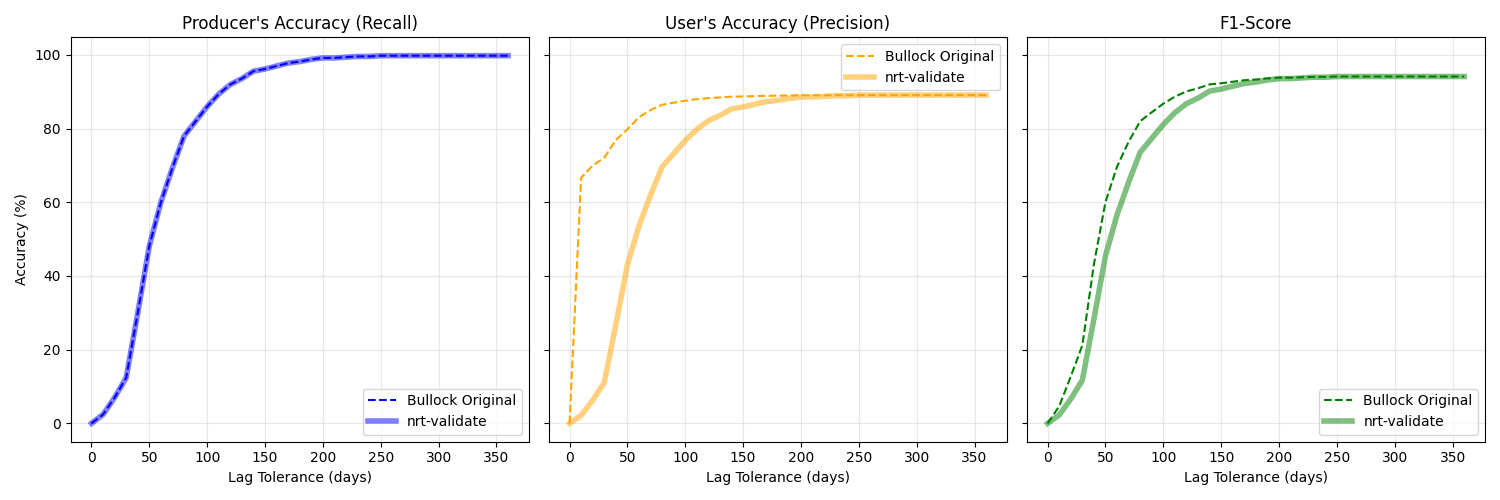
4. Visualization: Metric Comparison
Let’s visualize the three metrics side-by-side in separate panels to see exactly where the two methods align and diverge.
fig, axes = plt.subplots(1, 3, figsize=(15, 5), sharex=True, sharey=True)

# Producer's Accuracy (Recall)
axes[0].plot(lags, orig_producers, color='blue', linestyle='--', label="Bullock Original")
axes[0].plot(df_nrt['lag'], df_nrt['pa'] * 100, color='blue', linestyle='-', alpha=0.5, linewidth=4, label="nrt-validate")
axes[0].set_title("Producer's Accuracy (Recall)")
axes[0].set_xlabel("Lag Tolerance (days)")
axes[0].set_ylabel("Accuracy (%)")
axes[0].legend()
axes[0].grid(True, alpha=0.3)

# User's Accuracy (Precision)
axes[1].plot(lags, orig_users, color='orange', linestyle='--', label="Bullock Original")
axes[1].plot(df_nrt['lag'], df_nrt['ua'] * 100, color='orange', linestyle='-', alpha=0.5, linewidth=4, label="nrt-validate")
axes[1].set_title("User's Accuracy (Precision)")
axes[1].set_xlabel("Lag Tolerance (days)")
axes[1].legend()
axes[1].grid(True, alpha=0.3)

# F1-Score
axes[2].plot(lags, orig_f1s, color='green', linestyle='--', label="Bullock Original")
axes[2].plot(df_nrt['lag'], df_nrt['f1'] * 100, color='green', linestyle='-', alpha=0.5, linewidth=4, label="nrt-validate")
axes[2].set_title("F1-Score")
axes[2].set_xlabel("Lag Tolerance (days)")
axes[2].legend()
axes[2].grid(True, alpha=0.3)

plt.tight_layout()
plt.show()
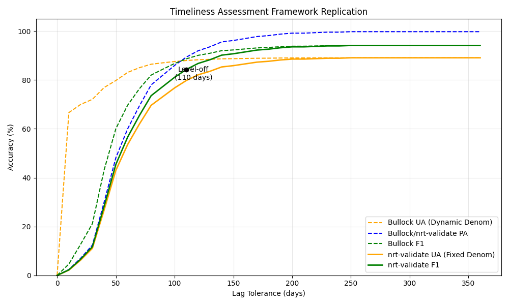
5. Extracting the “Level Off Point”
A major contribution of the Bullock paper is standardizing two metrics from
these curves: Initial Delay and Level-off point. nrt-validate provides
native helper functions for this.
initial_delay_lag, initial_delay_val = evaluator.find_initial_delay(df_nrt, metric='pa')
level_off_lag, level_off_val = evaluator.find_level_off(df_nrt, metric='f1', start_lag=int(initial_delay_lag))

print(f"Metrics evaluated by nrt-validate:")
print(f"  -> Initial Delay: {initial_delay_lag} days")
print(f"  -> Level-off Point: {level_off_lag} days")
Metrics evaluated by nrt-validate:
  -> Initial Delay: 10 days
  -> Level-off Point: 110 days
6. Visualization: The Denominator Effect
This final plot shows all metrics overlaid on a single axis. Because the fixed denominator in nrt-validate penalizes false alarms immediately, precision increases organically as the lag window expands to encompass correct, but delayed, detections.
fig, ax = plt.subplots(figsize=(10, 6))

# Plot Bullock Original
ax.plot(lags, orig_users, color='orange', linestyle='--', label="Bullock UA (Dynamic Denom)")
ax.plot(lags, orig_producers, color='blue', linestyle='--', label="Bullock/nrt-validate PA")
ax.plot(lags, orig_f1s, color='green', linestyle='--', label="Bullock F1")

# Plot nrt-validate
ax.plot(df_nrt['lag'], df_nrt['ua'] * 100, color='orange', linestyle='-', linewidth=2, label="nrt-validate UA (Fixed Denom)")
# PA is identical, so we don't plot the solid blue line over the dashed one.
ax.plot(df_nrt['lag'], df_nrt['f1'] * 100, color='green', linestyle='-', linewidth=2, label="nrt-validate F1")

# Annotate Level Off
if not np.isnan(level_off_lag):
    ax.scatter([level_off_lag], [level_off_val * 100], color='black', zorder=5)
    ax.annotate(f"Level-off\n({int(level_off_lag)} days)",
                (level_off_lag, level_off_val * 100),
                textcoords="offset points",
                xytext=(10,-15), ha='center')

ax.set_title("Timeliness Assessment Framework Replication")
ax.set_xlabel("Lag Tolerance (days)")
ax.set_ylabel("Accuracy (%)")
ax.set_ylim(0, 105)
ax.legend(loc="lower right")
ax.grid(True, alpha=0.3)

plt.tight_layout()
plt.show()
Total running time of the script: (0 minutes 0.439 seconds)