Spatial accuracy estimators

nrt-validate implements various accuracy estimators. This example demonstrates their use, comparing their precision and discussing trade-offs involved. Although nrt-validate has a strong focus on the temporal aspects of things, for greater separation of concerns this example is limited to the spatial accuracy aspects.

Validation Note: The results presented here have been validated against the R survey package to ensure statistical correctness of the point estimates and standard errors.

import numpy as np
import matplotlib.pyplot as plt
import matplotlib.colors as colors
import matplotlib.patches as mpatches
import pandas as pd
from scipy.ndimage import binary_dilation
from pprint import pprint

from nrt.data import simulate
from nrt.validate.estimators import (
    SimpleRandomEstimator,
    StratifiedEstimator,
    TwoStageClusterEstimator
)

# Set random seed for reproducibility
np.random.seed(42)

Create synthetic data with known accuracy

We utilize the nrt.data.simulate module to generate a synthetic landscape containing forest cover and disturbance events. We then simulate a monitoring system’s output (prediction) with specific error rates.

Because we generate the complete “Truth” and “Prediction” maps, we can calculate the exact, true accuracy metrics. This allows us to verify if the confidence intervals produced by our estimators correctly capture the true value and to compare the standard errors (precision) of different sampling designs.

# 1. Generate Landscape (Reference)
# 0=Non-Forest, 1=Forest, 2=Loss
land_cover, loss_dates = simulate.make_landscape(
    shape=(2000, 2000),
    year=2020,
    forest_pct=0.7,
    loss_pct=0.03, # 3% of landscape is loss
    seed=42
)

# 2. Generate Prediction
# 0=Stable, 1=Loss
pred_lc, pred_dates = simulate.make_prediction(
    land_cover,
    loss_dates,
    omission_rate=0.2,
    commission_rate=0.005,
    seed=42
)

# 3. Define the Validation Universe (Forest Only)
# We only assess accuracy within the forest mask. Non-forest areas are excluded.
forest_mask = land_cover > 0
# Flatten arrays for easier indexing within the forest domain
valid_idx = np.where(forest_mask.ravel())[0]

# Prepare flattened vectors for validation
# Reference: True if Loss (2), False if Stable Forest (1)
y_true_full = (land_cover.ravel()[valid_idx] == 2).astype(int)
# Prediction: True if Loss (1), False if Stable (0)
y_pred_full = (pred_lc.ravel()[valid_idx] == 1).astype(int)

# 4. Compute "True" Population Metrics
# We use a dummy estimator just to access the math methods on the full population
dummy_est = SimpleRandomEstimator()
true_oa, _ = dummy_est.overall_accuracy(y_true_full, y_pred_full)
true_ua, _ = dummy_est.user_accuracy(y_true_full, y_pred_full, label=1)
true_pa, _ = dummy_est.producer_accuracy(y_true_full, y_pred_full, label=1)
true_f1, _ = dummy_est.f1_score(y_true_full, y_pred_full, label=1)

print(f"TRUE POPULATION METRICS (Target for estimation):")
print(f"OA: {true_oa:.2%}, UA (Precision): {true_ua:.2%}, PA (Recall): {true_pa:.2%}, F1: {true_f1:.2%}")

# Dictionary to store results: {ScenarioName: {'UA': (est, se), 'PA': (est, se), 'F1': (est, se)}}
results = {}

# Define colormap for visualization: 0=Non-Forest (Tan), 1=Forest (Green), 2=Loss (Magenta)
cmap_lc = colors.ListedColormap(['#eecfa1', '#228b22', '#ff00ff'])

TRUE POPULATION METRICS (Target for estimation):
OA: 98.67%, UA (Precision): 87.76%, PA (Recall): 80.10%, F1: 83.76%

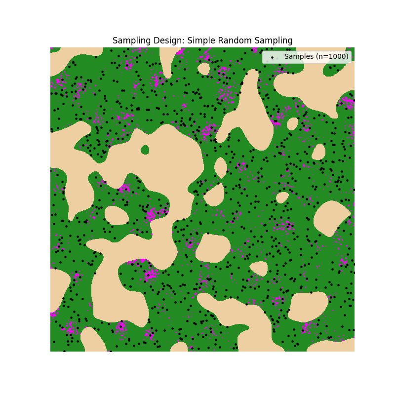
Scenario 1: Simple Random Sampling (SRS)

We select 1000 random pixels from the forest domain without any prior stratification. This serves as our baseline.

Estimator: SimpleRandomEstimator

This estimator is the simplest approach, assuming equal probability of selection for all pixels. We calculate metrics for label=1 (Loss class) specifically.

# Select 1000 random pixels from the forest domain
n_sample = 1000
sample_indices = np.random.choice(valid_idx, size=n_sample, replace=False)

# Get Reference and Prediction for samples
y_t_srs = (land_cover.ravel()[sample_indices] == 2).astype(int)
y_p_srs = (pred_lc.ravel()[sample_indices] == 1).astype(int)

est_srs = SimpleRandomEstimator()

# Calculate Metrics
ua, ua_se = est_srs.user_accuracy(y_t_srs, y_p_srs, label=1)
pa, pa_se = est_srs.producer_accuracy(y_t_srs, y_p_srs, label=1)
# Utilizing the built-in simple bootstrap for F1
f1, f1_se = est_srs.f1_score(y_t_srs, y_p_srs, label=1, se_method='bootstrap', n_boot=200)

results["SRS"] = {'UA': (ua, ua_se), 'PA': (pa, pa_se), 'F1': (f1, f1_se)}

# Visualize SRS
plt.figure(figsize=(8, 8))
plt.imshow(land_cover, cmap=cmap_lc, interpolation='none')
y_pts, x_pts = np.unravel_index(sample_indices, land_cover.shape)
plt.scatter(x_pts, y_pts, c='black', s=5, label='Samples (n=1000)')
plt.title("Sampling Design: Simple Random Sampling")
plt.axis('off')
plt.legend(loc='upper right')
plt.show()

Scenario 2: Post-stratification

We use the same samples as SRS, but we apply weights based on the map classes (strata) afterwards. This is known as post-stratification.

Estimator: StratifiedEstimator

Even though the design was simple random sampling, we can use the StratifiedEstimator by treating the map classes found at sample locations as strata.

Critical Arguments:

• strata_labels: The map class values extracted at the sample coordinates.

• stratum_pop_sizes: The total pixel count of each map class (Stable vs Loss) in the entire forest domain. These counts allow the estimator to calculate correct weights (\(N_h / n_h\)).

# We use the SAME sample as SRS, but we apply weights based on the map classes (strata).
# This usually reduces standard error compared to pure SRS.
map_strata = pred_lc.ravel()[sample_indices] # The map class of our samples
# Calculate population sizes (Nh) for the forest domain
# Class 0 (Stable) within Forest, Class 1 (Loss) within Forest
pop_counts = {
    0: np.sum((pred_lc.ravel() == 0) & forest_mask.ravel()),
    1: np.sum((pred_lc.ravel() == 1) & forest_mask.ravel())
}

est_post = StratifiedEstimator(strata_labels=map_strata, stratum_pop_sizes=pop_counts)

# Calculate Metrics (Analytic SE for UA/PA is standard for stratified)
ua, ua_se = est_post.user_accuracy(y_t_srs, y_p_srs, label=1)
pa, pa_se = est_post.producer_accuracy(y_t_srs, y_p_srs, label=1)
# Stratified estimator supports element-wise bootstrap correctly
f1, f1_se = est_post.f1_score(y_t_srs, y_p_srs, label=1, se_method='bootstrap', n_boot=200)

results["Post-Stratified"] = {'UA': (ua, ua_se), 'PA': (pa, pa_se), 'F1': (f1, f1_se)}

Scenario 3: Stratified Random Sampling (Map Classes)

Here we stratify the population before sampling. We define two strata based on the prediction map: ‘Stable’ and ‘Loss’. We allocate samples equally (500 each).

Estimator: StratifiedEstimator

We use the same estimator as in Scenario 2.

Critical Arguments:

• strata_labels: In this design, these are the strata we targeted during sampling (Map Classes). Weights will be significantly different here because we forced \(n_{loss} = 500\) (over-sampling the rare class). The estimator handles this automatically via the population sizes.

# Strata: 0=Stable, 1=Loss. Allocation: Equal (500 each).
# This ensures we have enough samples in the rare "Loss" class.
n_stratum = 500
strata_map = pred_lc.ravel()

# Indices for each stratum within forest
idx_stable = valid_idx[strata_map[valid_idx] == 0]
idx_loss = valid_idx[strata_map[valid_idx] == 1]

samp_stable = np.random.choice(idx_stable, size=n_stratum, replace=False)
samp_loss = np.random.choice(idx_loss, size=n_stratum, replace=False)
sample_strat = np.concatenate([samp_stable, samp_loss])

y_t_strat = (land_cover.ravel()[sample_strat] == 2).astype(int)
y_p_strat = (pred_lc.ravel()[sample_strat] == 1).astype(int)
strata_labels = strata_map[sample_strat]

est_strat = StratifiedEstimator(strata_labels=strata_labels, stratum_pop_sizes=pop_counts)

# Calculate Metrics
ua, ua_se = est_strat.user_accuracy(y_t_strat, y_p_strat, label=1)
pa, pa_se = est_strat.producer_accuracy(y_t_strat, y_p_strat, label=1)
f1, f1_se = est_strat.f1_score(y_t_strat, y_p_strat, label=1, se_method='bootstrap', n_boot=200)

results["Stratified (Map)"] = {'UA': (ua, ua_se), 'PA': (pa, pa_se), 'F1': (f1, f1_se)}

Scenario 4: Stratified Sampling (Map + Buffer)

We refine our stratification by adding a “Buffer” stratum around predicted loss. This targets the areas most prone to omission errors or spatial mismatches.

Estimator: StratifiedEstimator

Again, we use the StratifiedEstimator.

Critical Arguments:

• strata_labels: Now contains three values (0=Stable, 1=Loss, 2=Buffer).

• stratum_pop_sizes: Must reflect the areas of Stable, Loss, and Buffer strata respectively. Note how pop_buffer is calculated to exclude the loss pixels themselves.

# Create a 3rd stratum: Buffer around loss (likely omission area).
# Dilate prediction (Loss=1) by 5 pixels
pred_loss_mask = (pred_lc == 1)
buffer_mask = binary_dilation(pred_loss_mask, iterations=5) & (~pred_loss_mask) & forest_mask

# Define Strata Map: 1=Loss, 2=Buffer, 0=Stable Background
strat_layer = np.zeros_like(pred_lc, dtype=int)
strat_layer[pred_lc == 1] = 1
strat_layer[buffer_mask] = 2
# Mask out non-forest for sampling logic
valid_mask = forest_mask.ravel()
strat_flat = strat_layer.ravel()

# Population sizes
pop_buffer = {
    0: np.sum((strat_layer == 0) & forest_mask),
    1: np.sum((strat_layer == 1) & forest_mask),
    2: np.sum((strat_layer == 2) & forest_mask)
}

# Allocation: ~333 each
n_per = 333
s_0 = np.random.choice(valid_idx[strat_flat[valid_idx] == 0], n_per)
s_1 = np.random.choice(valid_idx[strat_flat[valid_idx] == 1], n_per)
s_2 = np.random.choice(valid_idx[strat_flat[valid_idx] == 2], n_per)
sample_buff = np.concatenate([s_0, s_1, s_2])

y_t_buff = (land_cover.ravel()[sample_buff] == 2).astype(int)
y_p_buff = (pred_lc.ravel()[sample_buff] == 1).astype(int)
strata_labels_buff = strat_flat[sample_buff]

est_buff = StratifiedEstimator(strata_labels=strata_labels_buff, stratum_pop_sizes=pop_buffer)

# Calculate Metrics
ua, ua_se = est_buff.user_accuracy(y_t_buff, y_p_buff, label=1)
pa, pa_se = est_buff.producer_accuracy(y_t_buff, y_p_buff, label=1)
f1, f1_se = est_buff.f1_score(y_t_buff, y_p_buff, label=1, se_method='bootstrap', n_boot=200)

results["Stratified (Buffer)"] = {'UA': (ua, ua_se), 'PA': (pa, pa_se), 'F1': (f1, f1_se)}

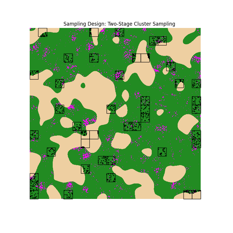
Scenario 5: Two-Stage Cluster Sampling (SRS at Stage 1)

Instead of picking individual pixels, we first select Primary Sampling Units (PSUs) which are 100x100 pixel blocks. Then, we sample pixels (SSUs) within these blocks.

Estimator: TwoStageClusterEstimator

This estimator handles the complex variance structure where pixels within a block are correlated.

Critical Arguments:

• psu_ids: Identifies which block each sample belongs to. Needed for cluster-level bootstrapping.

• global_weights: The combined weight of Stage 1 selection (PSU) and Stage 2 selection (SSU).

Understanding Weights in Two-Stage Sampling with Domain Estimation

When we sample a sub-population (Forests) within a larger frame (Total Area), we must adjust weights to reflect that the “population size” of a cluster is its forest area, not its total area.

The weight for a sampled pixel (SSU) is the product of two probabilities:

1. Stage 1 Weight (PSU Level): Inverse probability of selecting the Cluster.

   \[w_1 = \frac{\text{Total Clusters}}{\text{Sampled Clusters}}\]

2. Stage 2 Weight (SSU Level): Inverse probability of selecting the Pixel GIVEN the cluster was selected.

   \[w_2 = \frac{\text{Total Forest Pixels in Cluster}}{\text{Sampled Forest Pixels in Cluster}}\]

   Note: If a cluster has 10,000 pixels but only 50 are Forest, and we sample 20 of those forest pixels: \(w_2 = 50 / 20 = 2.5\) (Each sample represents 2.5 forest pixels). If we used total pixels (10,000/20), we would drastically overestimate.

# Primary Sampling Units (PSUs): 100x100 pixel blocks
# Grid Setup
H, W = land_cover.shape
block_size = 100
# Create PSU Map
y_grid, x_grid = np.indices((H, W))
psu_map = (y_grid // block_size) * (W // block_size) + (x_grid // block_size)
psu_flat = psu_map.ravel()

# Select 50 clusters randomly
all_psus = np.unique(psu_flat)
selected_psus = np.random.choice(all_psus, 50, replace=False)

# Select 20 SSUs per cluster (or all available forest pixels)
sample_cluster_idx = []
actual_psu_ids = []
weights_cluster = []

# Global weight stage 1
w_stage1 = len(all_psus) / 50

for psu in selected_psus:
    # Candidates in this PSU that are Forest (optimized using valid_idx for speed)
    candidates = valid_idx[psu_flat[valid_idx] == psu]
    pop_forest_in_psu = len(candidates)

    if pop_forest_in_psu > 0:
        n_take = min(20, pop_forest_in_psu)
        picked = np.random.choice(candidates, n_take, replace=False)

        sample_cluster_idx.append(picked)
        actual_psu_ids.extend([psu] * n_take)

        # Domain Estimation Weighting
        w_stage2 = pop_forest_in_psu / n_take
        w_final = w_stage1 * w_stage2
        weights_cluster.extend([w_final] * n_take)

sample_cluster_idx = np.concatenate(sample_cluster_idx)
actual_psu_ids = np.array(actual_psu_ids)
y_t_clus = (land_cover.ravel()[sample_cluster_idx] == 2).astype(int)
y_p_clus = (pred_lc.ravel()[sample_cluster_idx] == 1).astype(int)

# strata_1_ids = zeros because no stage 1 stratification
est_clus = TwoStageClusterEstimator(
    psu_ids=actual_psu_ids,
    strata_1_ids=np.zeros_like(actual_psu_ids),
    global_weights=np.array(weights_cluster),
    n_boot=200,
    se_method='bootstrap' # Using bootstrap SE
)

# Calculate Metrics
# TwoStageClusterEstimator supports UA/PA estimation (via ratio estimation) with bootstrap variance
ua, ua_se = est_clus.user_accuracy(y_t_clus, y_p_clus, label=1)
pa, pa_se = est_clus.producer_accuracy(y_t_clus, y_p_clus, label=1)
# Now utilizing the built-in bootstrap method
f1, f1_se = est_clus.f1_score(y_t_clus, y_p_clus, label=1, se_method='bootstrap', n_boot=200)

results["Cluster (SRS)"] = {'UA': (ua, ua_se), 'PA': (pa, pa_se), 'F1': (f1, f1_se)}

# Visualize Clusters
plt.figure(figsize=(8, 8))
plt.imshow(land_cover, cmap=cmap_lc, interpolation='none')
ax = plt.gca()

# Draw PSU Squares
unique_psus = np.unique(actual_psu_ids)
W_blocks = W // block_size
for psu in unique_psus:
    row = psu // W_blocks
    col = psu % W_blocks
    rect = mpatches.Rectangle((col * block_size, row * block_size), block_size, block_size,
                              linewidth=1, edgecolor='black', facecolor='none')
    ax.add_patch(rect)

# Draw SSU Samples
y_pts, x_pts = np.unravel_index(sample_cluster_idx, land_cover.shape)
plt.scatter(x_pts, y_pts, c='black', s=2)
plt.title("Sampling Design: Two-Stage Cluster Sampling")
plt.axis('off')
plt.show()

Scenario 6: Two-Stage Cluster (Stratified Stage 1)

We improve the cluster sampling by stratifying the Stage 1 (PSUs). We classify blocks into “High Disturbance” and “Low Disturbance” based on the prediction map. We then sample blocks from both strata to ensure we capture areas of interest.

Note on Stratification: The stratification used for Stage 1 selection can be based on any ancillary data, such as administrative boundaries (e.g., states/provinces), disturbance intensity (as shown here), or biogeographic regions. The goal is to group similar PSUs to reduce variance.

Estimator: TwoStageClusterEstimator

Critical Arguments:

• strata_1_ids: Crucial addition here. It tells the estimator that PSUs were selected from different strata (Low vs High intensity). The bootstrap resampling will respect these strata (resampling PSUs within their stratum) to correctly estimate variance.

# Stratify PSUs based on "Disturbance Intensity" (sum of prediction)
psu_intensity = {}
for p in all_psus:
    # Count predicted loss pixels in this PSU
    mask_p = (psu_flat == p)
    loss_count = np.sum(pred_lc.ravel()[mask_p] == 1)
    psu_intensity[p] = loss_count

intensities = np.array(list(psu_intensity.values()))
median_int = np.median(intensities[intensities > 0]) # Median of non-zero blocks

# Define PSU Strata: 0=Low/None, 1=High
psu_strata_dict = {p: (1 if val > median_int else 0) for p, val in psu_intensity.items()}
psu_strata_list = np.array([psu_strata_dict[p] for p in all_psus])

# Sample 25 PSUs from Low, 25 from High
psus_low = all_psus[psu_strata_list == 0]
psus_high = all_psus[psu_strata_list == 1]
N_low = len(psus_low)
N_high = len(psus_high)

sel_low = np.random.choice(psus_low, 25, replace=False)
sel_high = np.random.choice(psus_high, 25, replace=False)
selected_psus_s = np.concatenate([sel_low, sel_high])

# Sample SSUs
sample_cls_idx = []
act_psu_ids_s = []
s1_ids_s = []
weights_cls = []

for psu in selected_psus_s:
    s_label = psu_strata_dict[psu]
    w1 = N_high / 25 if s_label == 1 else N_low / 25
    candidates = valid_idx[psu_flat[valid_idx] == psu]
    pop_forest_in_psu = len(candidates)

    if pop_forest_in_psu > 0:
        n_take = min(20, pop_forest_in_psu)
        picked = np.random.choice(candidates, n_take, replace=False)
        w2 = pop_forest_in_psu / n_take
        w_final = w1 * w2

        sample_cls_idx.append(picked)
        act_psu_ids_s.extend([psu] * n_take)
        s1_ids_s.extend([s_label] * n_take)
        weights_cls.extend([w_final] * n_take)

sample_cls_idx = np.concatenate(sample_cls_idx)
act_psu_ids_s = np.array(act_psu_ids_s)
s1_ids_s = np.array(s1_ids_s)

y_t_cls = (land_cover.ravel()[sample_cls_idx] == 2).astype(int)
y_p_cls = (pred_lc.ravel()[sample_cls_idx] == 1).astype(int)

est_clus_s = TwoStageClusterEstimator(
    psu_ids=act_psu_ids_s,
    strata_1_ids=s1_ids_s,
    global_weights=np.array(weights_cls),
    n_boot=200,
    se_method='bootstrap'
)

# Calculate Metrics
ua, ua_se = est_clus_s.user_accuracy(y_t_cls, y_p_cls, label=1)
pa, pa_se = est_clus_s.producer_accuracy(y_t_cls, y_p_cls, label=1)
# Use custom cluster bootstrap for F1
f1, f1_se = est_clus_s.f1_score(y_t_cls, y_p_cls, label=1, se_method='bootstrap', n_boot=200)

results["Cluster (Strat)"] = {'UA': (ua, ua_se), 'PA': (pa, pa_se), 'F1': (f1, f1_se)}

pprint(results)

{'Cluster (SRS)': {'F1': (np.float64(0.7428603700004754),
                          np.float64(0.04700806026189324)),
                   'PA': (np.float64(0.7341836854598012),
                          np.float64(0.05903871998630786)),
                   'UA': (np.float64(0.7517445917655268),
                          np.float64(0.06739608564375651))},
 'Cluster (Strat)': {'F1': (np.float64(0.8235952884767413),
                            np.float64(0.05873744307830703)),
                     'PA': (np.float64(0.8046963149754535),
                            np.float64(0.07521909874568274)),
                     'UA': (np.float64(0.8434033289360118),
                            np.float64(0.07258429537118673))},
 'Post-Stratified': {'F1': (np.float64(0.7474004615318642),
                            np.float64(0.050242612814772915)),
                     'PA': (np.float64(0.6740207156067383),
                            np.float64(0.05726048426816362)),
                     'UA': (np.float64(0.8387096774193549),
                            np.float64(0.06714101193761311))},
 'SRS': {'F1': (np.float64(0.7123287671232876),
                np.float64(0.06074007686391275)),
         'PA': (np.float64(0.6190476190476191),
                np.float64(0.07584124375059005)),
         'UA': (np.float64(0.8387096774193549),
                np.float64(0.06715051611181072))},
 'Stratified (Buffer)': {'F1': (np.float64(0.8353764324170848),
                                np.float64(0.01929641269520688)),
                         'PA': (np.float64(0.7927214194193763),
                                np.float64(0.031806607575434714)),
                         'UA': (np.float64(0.882882882882883),
                                np.float64(0.017621036412545237))},
 'Stratified (Map)': {'F1': (np.float64(0.8725578038777775),
                             np.float64(0.03293010015693545)),
                      'PA': (np.float64(0.8576435030035312),
                             np.float64(0.07036805764019087)),
                      'UA': (np.float64(0.8880000000000001),
                             np.float64(0.0140854783939595))}}

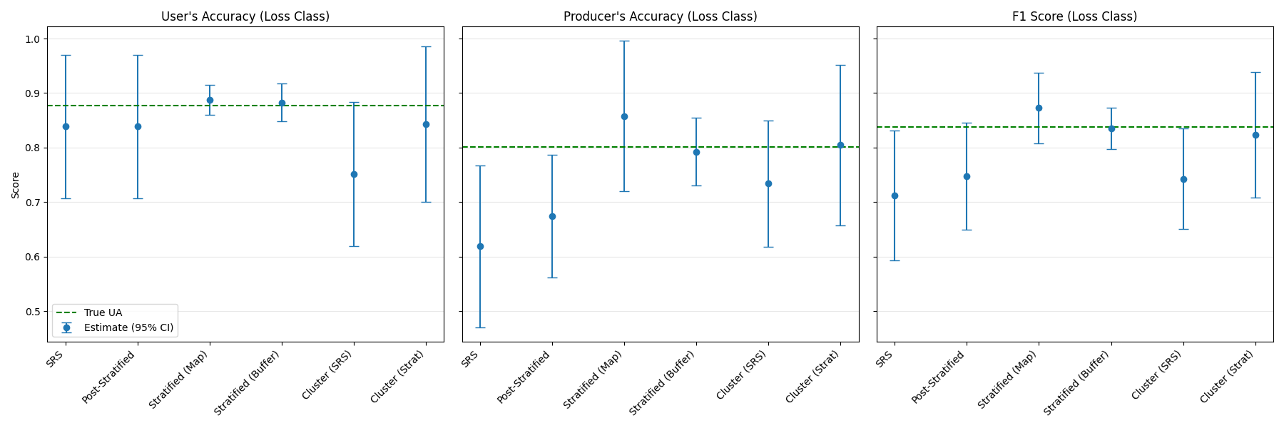
Visualize differences in precision

Here we plot the estimated metrics and their 95% confidence intervals against the True Population values.

Comparison of estimators:

1. SRS vs. Post-Stratification: # You may notice that the Confidence Intervals (CI) for User’s Accuracy (UA) are nearly identical between these two. This is expected when strata are defined by the map classes. UA is the probability that a pixel mapped as “Loss” is truly “Loss”. In post-stratification, this calculation relies almost entirely on samples within the “Loss” stratum. Since we use the exact same samples as SRS, the effective sample size for this specific metric is the same, leading to similar precision. Post-stratification typically offers greater precision gains for area estimates or Overall Accuracy.

2. Stratified Sampling (Buffer): # This scenario often yields the highest precision (narrowest CIs). By defining a specific stratum for the “uncertainty zone” (buffers around detections), we allocate more samples to where errors (especially spatial mismatch and omissions) are most likely, reducing the variance of the Producer’s Accuracy and F1 Score.

3. Cluster Sampling & Trade-offs: Two-Stage Cluster sampling shows wider confidence intervals than Stratified Random sampling for the same total number of pixels (\(n=1000\)). This is due to the “Design Effect”: pixels within the same cluster are correlated, so 1000 clustered pixels contain less unique information than 1000 independent ones.

   Why use Cluster Sampling then? Despite lower statistical efficiency per pixel, it may be preferred for:

   • Field Logistics: Minimizes travel time by grouping sample points.

   • Cost Efficiency: If validation relies on purchasing expensive VHR imagery, buying 50 large blocks is often cheaper or more feasible than 1000 tiny, scattered chips.

   • Algorithm Development: It facilitates testing new algorithms. You only need to process the data for the selected clusters (e.g., 50 blocks) rather than the entire continental scale, allowing for rapid iteration and “intercomparison” of approaches without generating wall-to-wall maps.

# Prepare Data for Plotting
metrics = ['UA', 'PA', 'F1']
true_vals = {'UA': true_ua, 'PA': true_pa, 'F1': true_f1}
metric_titles = {'UA': "User's Accuracy (Loss Class)", 'PA': "Producer's Accuracy (Loss Class)", 'F1': "F1 Score (Loss Class)"}
scenarios = list(results.keys())

fig, axes = plt.subplots(1, 3, figsize=(18, 6), sharey=True)

for i, m in enumerate(metrics):
    ax = axes[i]

    # Extract Estimates and SEs
    estimates = [results[s][m][0] for s in scenarios]
    se_values = [results[s][m][1] for s in scenarios]

    # Calculate 95% Confidence Intervals
    cis = [1.96 * se for se in se_values]

    # Plot
    ax.errorbar(scenarios, estimates, yerr=cis, fmt='o', capsize=5, label='Estimate (95% CI)')
    ax.axhline(true_vals[m], color='green', linestyle='--', label=f'True {m}')
    ax.set_title(metric_titles[m])
    ax.set_xticklabels(scenarios, rotation=45, ha='right')
    ax.grid(axis='y', alpha=0.3)
    if i == 0:
        ax.set_ylabel('Score')
        ax.legend()

plt.tight_layout()
plt.show()

/home/docs/checkouts/readthedocs.org/user_builds/nrt-validate/checkouts/latest/docs/gallery/plot_spatial_accuracy_estimators.py:550: UserWarning: set_ticklabels() should only be used with a fixed number of ticks, i.e. after set_ticks() or using a FixedLocator.
  ax.set_xticklabels(scenarios, rotation=45, ha='right')
/home/docs/checkouts/readthedocs.org/user_builds/nrt-validate/checkouts/latest/docs/gallery/plot_spatial_accuracy_estimators.py:550: UserWarning: set_ticklabels() should only be used with a fixed number of ticks, i.e. after set_ticks() or using a FixedLocator.
  ax.set_xticklabels(scenarios, rotation=45, ha='right')
/home/docs/checkouts/readthedocs.org/user_builds/nrt-validate/checkouts/latest/docs/gallery/plot_spatial_accuracy_estimators.py:550: UserWarning: set_ticklabels() should only be used with a fixed number of ticks, i.e. after set_ticks() or using a FixedLocator.
  ax.set_xticklabels(scenarios, rotation=45, ha='right')

Going further

These estimators are designed to be interoperable with the metrics module. While this example focused on spatial aggregates, future updates will demonstrate linking these estimators with temporal lag curves to produce accuracy-with-confidence plots for time-series monitoring.