Temporal accuracy metrics

This example demonstrates how to evaluate the timeliness of a monitoring system.

Unlike spatial accuracy (which asks “is the map correct?”), temporal accuracy asks: “How quickly does the system detect changes?”

This tutorial will guide you through: 1. Generating synthetic disturbance data with known dates. 2. Computing the True accuracy curves using the exhaustive dataset (as a benchmark). 3. Sampling points using a stratified design to capture enough disturbance events. 4. Using TemporalEvaluator to estimate accuracy curves from the sample. 5. Calculating key metrics like Initial Delay and Level-off Point.

import numpy as np
import pandas as pd
import matplotlib.pyplot as plt
from nrt.data import simulate
from nrt.validate.metrics import TemporalEvaluator
from nrt.validate.estimators import StratifiedEstimator, SimpleRandomEstimator

# Set random seed for reproducibility
np.random.seed(42)

1. Generate Synthetic Temporal Data

We simulate a landscape where disturbances happen at specific dates. The monitoring system detects these with some delay and occasional errors.

• Reference Dates: When the disturbance actually occurred.

• Prediction Dates: When the system flagged the pixel.

# 1. Landscape & Reference Dates
# 0=Non-Forest, 1=Forest, 2=Loss
land_cover, loss_dates = simulate.make_landscape(
    shape=(1000, 1000),
    year=2021,
    forest_pct=0.8,
    loss_pct=0.05,
    seed=42
)

# 2. Prediction & Detection Dates
# Simulating a system with:
# - Good detection rate (low omission)
# - Variable delays (some fast, some slow)
pred_lc, pred_dates = simulate.make_prediction(
    land_cover,
    loss_dates,
    omission_rate=0.1,
    commission_rate=0.01,
    seed=42
)

# Mask valid forest universe
forest_mask = land_cover > 0
valid_idx = np.where(forest_mask.ravel())[0]

# Flatten arrays for sampling
y_true_dates = loss_dates.ravel()
y_pred_dates = pred_dates.ravel()
y_pred_class = pred_lc.ravel()  # 0=Stable, 1=Loss

# Determine temporal bounds dynamically from the data.
# This ensures robust handling whether the simulation returns Day-of-Year (1-365)
# or Days-Since-Epoch.
valid_dates = y_true_dates[y_true_dates > 0]
if len(valid_dates) > 0:
    exp_start = int(valid_dates.min())
    exp_end = int(valid_dates.max())
else:
    # Fallback if no loss generated
    exp_start, exp_end = 1, 365

print(f"Temporal Experiment Window: {exp_start} to {exp_end}")

Temporal Experiment Window: 18628 to 18992

2. Compute True Accuracy Curves

In a simulation, we have access to the full “Truth”. We can calculate the exact temporal accuracy curves by evaluating every single pixel. This serves as a ground truth to verify our sample-based estimates later.

We use the TemporalEvaluator with a SimpleRandomEstimator. When applied to the entire population without sampling, this calculates the true population parameters.

# We apply the evaluator to the full flattened arrays (valid forest pixels only)
y_true_full = y_true_dates[valid_idx]
y_pred_full = y_pred_dates[valid_idx]

true_evaluator = TemporalEvaluator(
    y_true=y_true_full,
    y_pred=y_pred_full,
    estimator=SimpleRandomEstimator(),
    experiment_start=exp_start,
    experiment_end=exp_end
)

lags = list(range(0, 101, 5))
df_true = true_evaluator.compute_curve(lags=lags, metrics=['ua', 'pa', 'f1'])

print(f"True F1 at lag 30: {df_true.loc[df_true['lag'] == 30, 'f1'].values[0]:.3f}")

True F1 at lag 30: 0.733

3. Stratified Sampling

In real-world scenarios, validating every pixel is impossible. We must sample. Temporal analysis requires a sufficient number of detected changes to build reliable curves. A simple random sample might not pick enough disturbances.

We use Stratified Random Sampling based on the prediction map:

• Stratum 1 (Detected Loss): 800 samples. (Heavily oversampled to capture timing dynamics).

• Stratum 0 (Stable): 200 samples. (To monitor false alarms).

# Define Strata based on Prediction Map
strata_map = y_pred_class
idx_loss = valid_idx[strata_map[valid_idx] == 1]
idx_stable = valid_idx[strata_map[valid_idx] == 0]

# Allocate Samples
n_loss = 800
n_stable = 200

samp_loss = np.random.choice(idx_loss, size=n_loss, replace=False)
samp_stable = np.random.choice(idx_stable, size=n_stable, replace=False)
sample_indices = np.concatenate([samp_loss, samp_stable])

# Extract Data for Samples
sample_true_dates = y_true_dates[sample_indices]
sample_pred_dates = y_pred_dates[sample_indices]
sample_strata = strata_map[sample_indices]

# Calculate Population Weights
# Essential for correcting the bias introduced by oversampling the Loss stratum.
pop_counts = {
    0: np.sum((strata_map == 0) & forest_mask.ravel()),
    1: np.sum((strata_map == 1) & forest_mask.ravel())
}

# Initialize Estimator
# This handles the weighting logic for us
estimator = StratifiedEstimator(
    strata_labels=sample_strata,
    stratum_pop_sizes=pop_counts
)

4. Estimated Temporal Evaluation

We initialize the TemporalEvaluator with our sample and the Stratified Estimator.

It allows us to ask: “What is the accuracy if we allow a delay of X days?”

evaluator = TemporalEvaluator(
    y_true=sample_true_dates,
    y_pred=sample_pred_dates,
    estimator=estimator,
    experiment_start=exp_start,
    experiment_end=exp_end
)

# Compute Accuracy Curves
# We evaluate User's Accuracy (UA), Producer's Accuracy (PA), and F1 Score
df_curve = evaluator.compute_curve(lags=lags, metrics=['ua', 'pa', 'f1'])
print(df_curve.head())

   lag        ua        pa        f1
0    0  0.000000  0.000000  0.000000
1    5  0.161388  0.143085  0.151686
2   10  0.398190  0.353033  0.374254
3   15  0.579186  0.513502  0.544370
4   20  0.704374  0.624493  0.662033

5. Key Metrics: Initial Delay & Level-off

Curves are informative, but single numbers are often needed to benchmark systems.

• Initial Delay: How long does it take to start detecting anything meaningful?

  (Defined as the lag where Producer’s Accuracy > 2%).

• Level-off Point: At what lag does accuracy stop improving significantly?

  (Found using the “Kneedle” algorithm on the F1 curve).

# Calculate Initial Delay (based on PA)
init_delay_lag, init_delay_val = evaluator.find_initial_delay(df_curve, metric='pa')

# Handle case where threshold is never reached (returns NaN)
start_lag_for_knee = 0
if not np.isnan(init_delay_lag):
    start_lag_for_knee = int(init_delay_lag)

# Calculate Level-off Point (based on F1)
# We start searching after the initial delay to avoid early noise
level_off_lag, level_off_val = evaluator.find_level_off(df_curve, metric='f1', start_lag=start_lag_for_knee)

print(f"Initial Delay: {init_delay_lag} days (PA={init_delay_val:.2f})")
print(f"Level-off:     {level_off_lag} days (F1={level_off_val:.2f})")

Initial Delay: 5 days (PA=0.14)
Level-off:     25 days (F1=0.72)

6. Visualization and Discussion

We plot the estimated metrics against the True population curves calculated in Step 2.

• Solid Lines: Estimated values from our stratified sample.

• Dotted Lines: True values from the exhaustive population.

Notice how the stratified estimator successfully recovers the true population dynamics despite the heavy oversampling of the disturbed class. Without the weights provided by StratifiedEstimator, the results would be heavily biased.

plt.figure(figsize=(10, 6))

# Plot Estimated Curves
plt.plot(df_curve['lag'], df_curve['f1'], label='Estimated F1', color='green', linewidth=2)
plt.plot(df_curve['lag'], df_curve['pa'], label="Estimated PA", color='blue', linestyle='--')
plt.plot(df_curve['lag'], df_curve['ua'], label="Estimated UA", color='orange', linestyle='--')

# Plot True Curves (Ground Truth)
plt.plot(df_true['lag'], df_true['f1'], label='True F1', color='green', linestyle=':', alpha=0.6)
plt.plot(df_true['lag'], df_true['pa'], label="True PA", color='blue', linestyle=':', alpha=0.6)
plt.plot(df_true['lag'], df_true['ua'], label="True UA", color='orange', linestyle=':', alpha=0.6)

# Mark Metrics
if not np.isnan(level_off_lag):
    plt.axvline(level_off_lag, color='grey', linestyle=':', alpha=0.7)
    plt.scatter([level_off_lag], [level_off_val], color='green', zorder=5)
    plt.text(level_off_lag + 2, level_off_val - 0.05,
             f'Level-off\n({int(level_off_lag)} days)', color='green')

if not np.isnan(init_delay_lag):
    plt.scatter([init_delay_lag], [init_delay_val], color='blue', zorder=5)
    plt.text(init_delay_lag + 2, init_delay_val + 0.02,
             f'Initial Delay\n({int(init_delay_lag)} days)', color='blue')

plt.xlabel('Temporal Lag Tolerance (days)')
plt.ylabel('Accuracy Metric')
plt.title('Time-to-Detection: Estimated vs True')
plt.legend(loc='lower right')
plt.grid(True, alpha=0.3)
plt.ylim(0, 1.0)
plt.show()

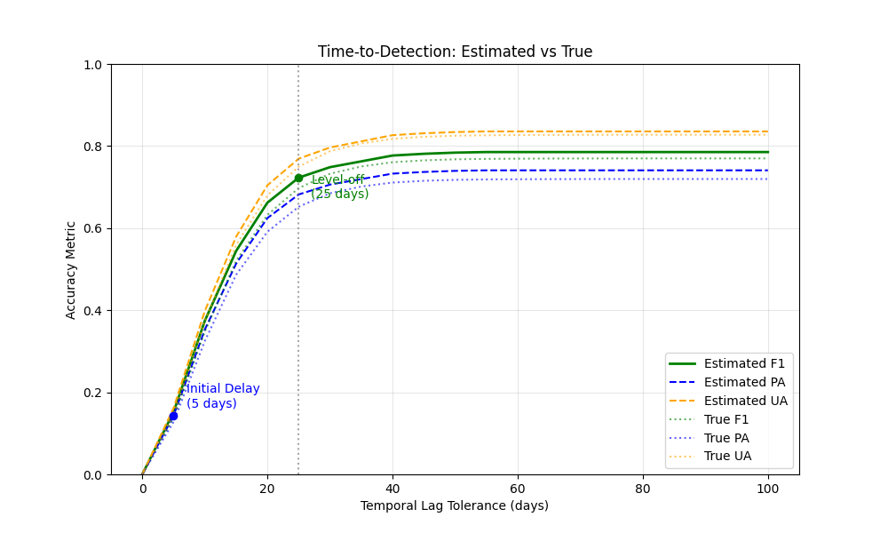
Interpretation

• Convergence: The estimated curves (solid) closely track the true curves (dotted),

  validating our sampling and estimation strategy.

• Rapid Rise: The steep slope at the beginning indicates that most disturbances

  are detected relatively quickly.

• Plateau: The curve flattens out (Level-off) when adding more “patience”

  (lag tolerance) no longer yields better accuracy. This suggests that remaining errors are likely permanent (e.g., missed events) rather than just late detections.